The collection nobody documented: meeting a legacy MongoDB with an AI agent

You join a team. There’s a collection called users. It’s been in production for years, nobody who designed it is still around, and there is no schema file — because MongoDB never made anyone write one. The User model in the codebase has about a dozen fields. The live collection has 120,000 documents and 27 distinct field paths, half of them added by migrations, A/B tests, and “just ship it” Fridays that nobody wrote down.

You’ve been asked to do three things this week:

1. Add a feature that touches this collection — so you need to know what’s actually in it.
2. Answer a compliance question: “where do we store personal data, and under which regulation?”
3. Figure out why a “list recent users” screen got slow.

In a normal week, that’s days of mongosh, db.users.findOne() roulette, guessing field names, grepping migration scripts, and squinting at explain() output. The data is right there — but it’s shaped like a swamp, and the tooling makes you wade through it one bucket at a time.

This is the gap 3T MCP closes. It’s a Model Context Protocol server for MongoDB: you point an MCP-aware agent (Claude Desktop, Cursor, VS Code) at your clusters once, and the agent can browse, profile, and reason about your data through a fixed, safe set of tools. No queries get smuggled past it; no credentials leak into the chat. The agent does the wading. You read the conclusions.

Everything below is a real run against a real 120,000-document collection. The numbers, buckets, and query plans are the tools’ actual output, not illustrations.

Step 0: connect once

The agent reads connections from a local YAML config — no connection strings pasted into the chat, no credentials in the transcript.

connections: - id: local label: Local MongoDB uri: mongodb://localhost:27017

In production you’d point this at a read-only replica — the whole workflow below is read-only. Now the agent can see the local connection, and only that.

Step 1: “What am I even looking at?”

You start with the obvious question:

You: I’ve inherited the users collection in the app database (local connection) and there’s no documentation. Profile what’s actually in it: every field, how common it is, and its type. Flag anything stored as more than one type, or that only shows up in a tiny fraction of documents.

The agent calls analyze_schema — and this is where the swamp becomes a map. The tool samples the collection and returns a flat field inventory: every dotted field path, the share of documents that carry it, the type(s) each field takes, and the most common values per type.

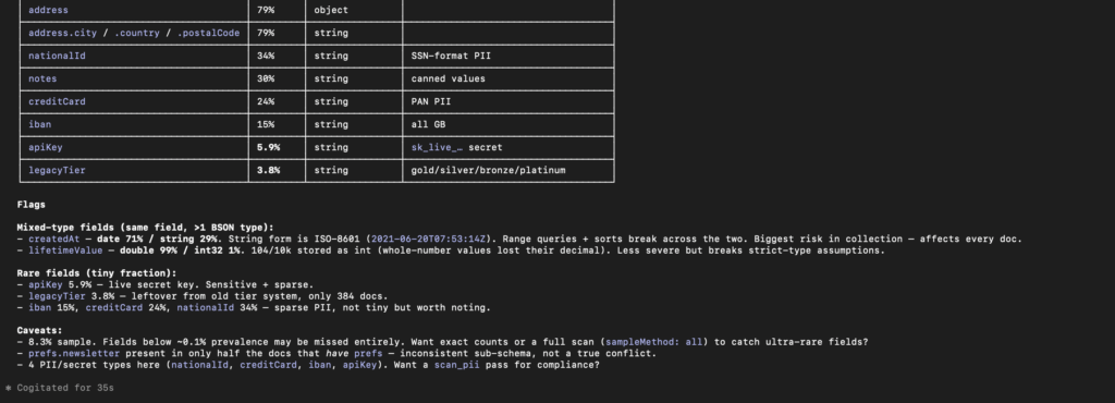
What comes back tells a story no model file could:

• email — present in 100% of documents, always a string. Fine.
• createdAt — present in 100%, but two types: date in ~72% of documents, string in ~28%. That’s a migration that never finished. A {createdAt: {$gte: someDate}} query silently skips more than a quarter of your users and never throws.
• lifetimeValue — double in 99%, but int32 in 1%. The same drift, quieter: a handful of rows where a whole-number value got stored as an integer. Enough to trip a strict deserializer.
• legacyTier — present in just ~4% of documents (bronze / silver / gold / platinum). A field you’d never find by reading findOne(), because the first documents don’t have it. It’s the residue of a pricing model from years ago that a couple of reports still depend on.
• prefs.marketingConsent — present in ~88%, boolean. Suddenly relevant to step 2.

The point isn’t that this data was hidden. It’s that getting it used to cost you an afternoon of ad-hoc aggregation, and now it costs you one sentence. The agent ran the sample, tallied the types, did the percentage math, and handed you the shape — including the two type-drift landmines you’d otherwise have stepped on in production.

// analyze_schema → app.users (excerpt) { "path": "createdAt", "probability": 1.0, "types": [ { "name": "date", "probability": 0.716 }, { "name": "string", "probability": 0.284 } ] } { "path": "lifetimeValue", "types": [ { "name": "double", "probability": 0.99 }, { "name": "int32", "probability": 0.01 } ] } { "path": "legacyTier", "probability": 0.039 } { "path": "prefs.marketingConsent", "probability": 0.881 }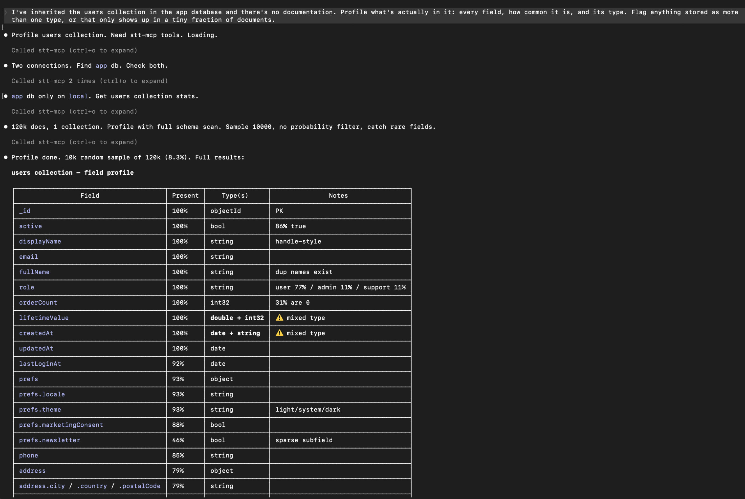

Step 2: “Where’s the personal data?”

Now the compliance question. Instead of grepping field names for email|phone|ssn and hoping, you ask:

You: Scan app.users for PII — what’s sensitive, which regulation, worst first. Just go by the scan’s results.

The agent calls scan_pii, which samples the collection, classifies every field by name and by value pattern, and sorts each into one of four buckets — Critical, PII, Potentially Sensitive, Likely Safe — with a confidence score, a suggested action, and a regulation hint per finding.

The first thing it surfaces is the one you most need to see — a single Critical finding:

// scan_pii → app.users { "field": "apiKey", "bucket": "Critical", "confidence": 1.0, "nameSignals": ["secret"], "occurrences": 275, "regulationHints": ["Credentials — should never be at rest in plaintext"], "suggestedAction": "remove or encrypt (client-side FLE / Queryable Encryption)" }

apiKey — a plaintext integration token, sitting on ~6% of user documents, left over from an old integration nobody remembers wiring up. No one would have gone looking for it. The scanner did, because the field name trips a secret signal, and a credential at rest in plaintext is the single most expensive thing this collection could be quietly carrying. That one finding can justify the whole exercise.

Then the regulated-but-routine personal data, the artifact you were dreading writing by hand:

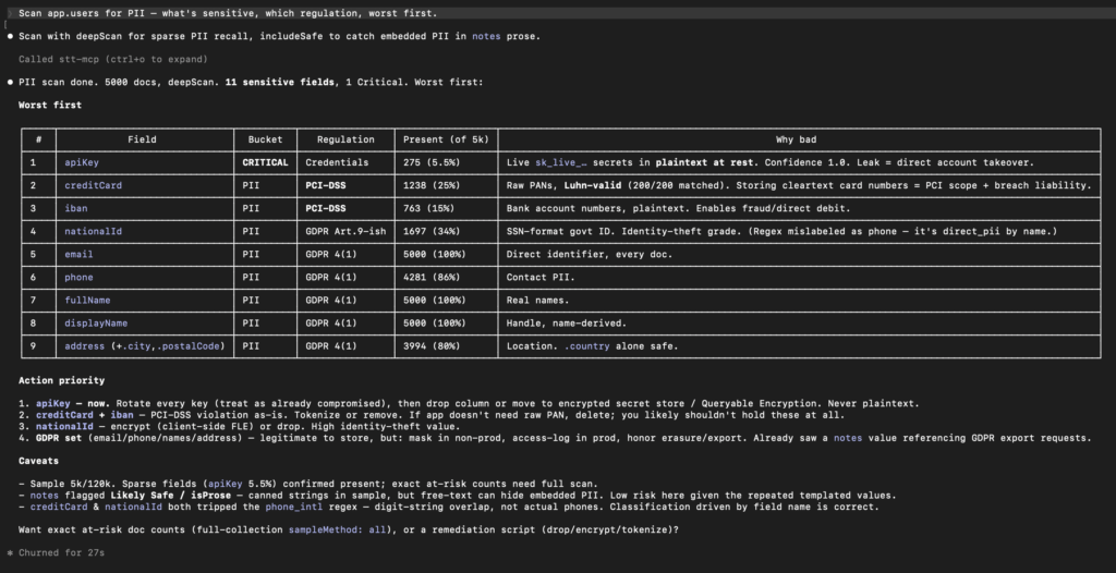
creditCard is the strong kind of finding — it isn’t trusting the field name, it’s matching the actual values (16 digits, Luhn-valid) and tagging them PCI-DSS. And note what it didn’t over-flag: address.country is just a two-letter code, left in Likely Safe rather than dragging the whole address subtree into the report. Sample values come back redacted — a***@proton.me, 4********4 — so the audit itself doesn’t spill what it’s auditing.

And then one more field comes back like this:

{ "field": "notes", "bucket": "Likely Safe", "confidence": 0.0, "occurrences": 2963, "isProse": true }

notes is a free-text field. Name-based and regex-based classification can’t bucket it — it’s prose, not a typed value — so the scanner doesn’t pretend to. What it does do is flag isProse: true: “this is a free-text column where personal data can hide, and I can’t see inside it for you. Go look.”

That flag is the whole game — and notice what the scanner didn’t do: it didn’t dump the contents of notes into the chat to prove its point. It can’t see inside prose, and it doesn’t pretend to, so it never spills what might be in there. It just tells you where to look, so you can route that field through a proper, access-logged review — instead of an audit that pulls years of support agents’ pasted-in customer emails and phone numbers straight into an LLM transcript. The most sensitive field in the collection is the one the tool is most careful with.

You paste the Critical finding, the table, and the notes flag into the compliance ticket and move on. That used to be a half-day audit.

Step 3: “Why is the recent-users screen slow?”

Last job. The screen lists recently registered active users: filter {active: true}, sort by {createdAt: -1}. You ask:

You: A screen that lists recently signed-up active users from app.users is slow. Look at that query — active users, newest first — and tell me whether it’s using an index or scanning the whole collection, and why it’s slow.

The agent calls explain_query (MongoDB explain with executionStats) and reads the plan back to you in English, not raw JSON:

No index supports this. The winning plan is a COLLSCAN feeding a blocking, in-memory SORT — it scans all 120,000 documents (totalKeysExamined: 0, totalDocsExamined: 120000) and sorts the matches in RAM on every request. That’s the source of your latency, and it gets worse linearly as the collection grows.

// explain_query → {active:true} sort {createdAt:-1} "winningPlan": { "stage": "SORT", "sortPattern": {"createdAt": -1}, "inputStage": { "stage": "COLLSCAN", "filter": {"active": {"$eq": true}} } } "totalKeysExamined": 0, "totalDocsExamined": 120000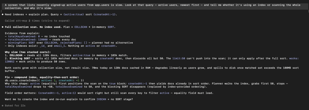

For contrast, you point it at a query that is indexed:

You: Now compare that to looking up a single user in app.users by their email address. Why is one fast and the other slow, and how would you fix the slow one?

The plan is the opposite: an IXSCAN on the unique email_1 index straight to a single FETCH, totalDocsExamined: 1. So the cluster isn’t un-indexed; this particular listing query just has nothing to lean on.

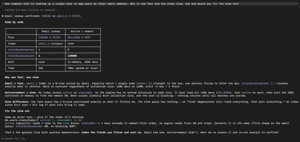
The fix is a compound index on {active: 1, createdAt: -1}, which turns the blocking sort into an index scan. But here’s where step 1 comes back to bite: ~28% of createdAt values are strings, not dates. Even with the index, MongoDB sorts strings and dates as separate type-brackets — so the “recently registered” list would be subtly wrong until that migration is finished. The agent flags it, because it already knows the field is split. You didn’t read a single line of raw explain() output, and you caught a bug the index alone wouldn’t have fixed.

What just happened

Three tasks. One chat session. No mongosh, no guessing field names, no afternoon lost to aggregation pipelines or explain() archaeology. The agent did the mechanical work — sampling, tallying, classifying, plan-reading — and you stayed at the level of decisions. Along the way it turned up a plaintext credential nobody knew was in the collection.

The reason this works, and works safely, is the boundary 3T MCP draws:

• The tool set is fixed and read-shaped. The agent can profile, classify, and explain. It calls a known set of tools — it can’t invent a dropDatabase. Business logic lives behind the tools, never in the prompt.
• Output is bounded and redacted. Query results are size- and count-capped so a curious agent can’t pull the whole collection into the chat, and scan_pii redacts sample values so an audit doesn’t become a leak.
• Credentials never touch the conversation. Connections live in local config; the agent sees connection ids, not secrets.

MongoDB’s flexibility is the feature that creates the swamp: no enforced schema means the data drifts, and the drift is invisible until it bites you. 3t-MCP gives an AI agent exactly the right instruments to walk into that swamp, profile it, and hand you back a map — schema reality, PII reality, and query reality — in the time it takes to ask three questions.

The collection nobody documented just documented itself.

Want to try this workflow? analyze_schema, scan_pii, and explain_query are three of the tools in 3T MCP. Install is a single command, the server runs entirely on your machine, and every tool is read-only — point it at a read replica and ask the three questions above about your oldest collection.

Get started with 3T MCP — setup takes under two minutes.