SQL Query

Basics

To open SQL Query:

• Button – Click on the SQL button on the global toolbar
• Right-click – Right-click on a collection and choose Open SQL
• Hotkey – Use Shift + Ctrl + L (Shift + ⌘+ L)

SQL Query has two main areas: the Editor at the top where you write SQL queries, and the Result tab at the bottom where query results and documents are shown.

SQL query auto-completion

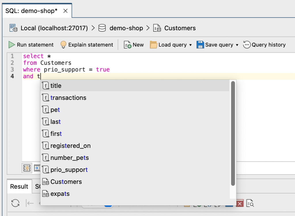
SQL Query supports smart auto-completion which is similar to auto-completion in IntelliShell, Studio 3T’s built-in shell for MongoDB. The editor detects and suggests standard SQL functions as well as fields, collections, and keyword names.

Run SQL queries and view the data

You can run a SQL statement in the following ways:

• Button – Click on the Run statement button
• Right-click – Place the cursor on the query, right-click, and choose Run SQL statement at cursor
• Hotkey – Press F5 to run the SQL statement at the cursor

The Result tab shows the MongoDB document data that matches your query. You can view the query results as rows and columns in Table View, in a hierarchical format in Tree View, or as scrollable JSON documents in JSON view.

Edit results inline

Editing documents and data in the SQL Query tab in Studio 3T is based on a ‘search and edit’ paradigm. Rather than searching for the documents you want to edit and then issuing separate UPDATE, DELETE, or INSERT commands, you simply edit the documents directly inline.

To edit a particular field or value in a document, simply double-click on it and Studio 3T will show a type-specific editor for that value.

Pressing ‘Enter’ writes the new value to the database, while pressing ‘Esc’ returns the previous value and exits the editor.

Read-only mode

To prevent accidental edits to document data, for example in a production database, you can enable read-only mode. Click on the padlock icon in the Result tab to stop the data being directly editable.

You can also configure read-only mode for all the databases and collections for a particular connection.

Open and save SQL queries

To save your SQL query so that you can use it throughout Studio 3T or as a .sql file:

• Button – Click on the Save query icon. Alternatively, click on the arrow to find the Save file functions.
• Right-click – Right-click anywhere in the Editor and choose Save
• Shortcuts – Save query – Ctrl + S (⌘+ S), Save file – Shift + Ctrl + S (Shift + ⌘+ S)

If you are using Studio 3T’s Team Sharing, you can save your SQL query in a shared folder. You and your team members can access the shared query from the My resources sidebar.

To store the connection, database, and collection details with your SQL query, select the Save target details checkbox.

To open existing .sql files, click Load query.

View query history

Whenever you run a query in Studio 3T, it is automatically saved. To view your query history, click Query history in the toolbar.

You can search through your history, save an item as a query so that you can use it again in Studio 3T, or load an existing query.

Generate JavaScript, Java, Python, C# and PHP code from SQL queries

Query Code converts SQL queries into JavaScript (Node.js), Java (2.x, 3.x, and 4.x driver API), Python, C#, PHP, and the MongoDB Shell language.

To see a SQL query’s equivalent code:

1. Run the SQL query.
2. Click on the Query Code tab.
3. Choose the target language.

View the equivalent MongoDB query

To learn how a SQL query translates to MongoDB query syntax:

1. Click on the Query Code tab.
2. If it isn’t already selected, choose MongoDB Shell.

Explain data for the query

Click Explain statement or simply click the Explain tab to open Visual Explain which shows you a visual flowchart of how MongoDB ran your query including the option to view execution statistics with Run full explain – a helpful tool for tuning your query’s performance.

Supported SQL expressions

To query MongoDB with SQL, Studio 3T supports many SQL-related expressions, functions, and methods to input a query. This tutorial uses the data set Customers to illustrate examples.

SELECT *

When you open SQL Query, Studio 3T automatically generates a basic SELECT * query by default. This retrieves all of the documents in a collection, similar to selecting all the rows of a table in an SQL database.

The SQL query

select *
from Customers;

shows all documents and fields in the Customers collection.

JSON objects in WHERE clauses

JSON can be used in SQL WHERE clauses in two ways:

WHERE JSON

or

WHERE identifier <SQL operator> JSON

JSON keys can be quoted or not. As strings, they can be quoted with single-quotes (”)  or double-quotes (“”), which means these two queries are the same:

SELECT * FROM [coordinates]
WHERE location = { "x" : 3 }

SELECT * FROM [coordinates]
WHERE { "location" : { "x" : 3 } }

You can also use a wide array of MongoDB data type constructors such as NumberInt, NumberLong, NumberDecimal, ObjectId, ISODate, Date, LUUID, CSUUID, JUUID, PYUUID, UUID, Timestamp, Symbol, DBRef, BinDate, and HexData.

Here are a few examples:

SELECT * FROM [binaries]
WHERE { "data" : BinData(3, '0x0') };

SELECT * FROM [table]
WHERE { 'date' : new Date(2019, 0, 2) }

This means we can also make use of any MongoDB operator.

SELECT * FROM [places]
WHERE {'$or' : [ { "item" : "foo" }, { 'item' : 'bar' } ] }

SELECT * FROM [words]
WHERE word = { $regex : "foo", "$options" : "i" }

SELECT DISTINCT

SELECT DISTINCT eliminates any repeated documents from the output.

Consider the query:

SELECT first_name FROM customers

It returns a table of names where the names can repeat:

Alice
Bob
Charlie
Bob
Charlie
...

But when you write the query with DISTINCT:

SELECT DISTINCT first_name FROM customers

you get a list of distinct names:

Alice
Bob
Charlie
...

So in a DISTINCT query output, each identical document is returned only once.

Note that all the SELECT-ed fields are taken into account. The query

SELECT DISTINCT first_name, last_name FROM customers

returns

Alice, Allen
Bob, Brown
Charlie, Clark
Alice, Brown
Bob, Clark
Charlie, Allen
...

First names and last names can repeat, but their pairs do not.

Technical restrictions to SELECT DISTINCT

When you have a query with DISTINCT and ORDER BY, you can sort only by a selected (visible) field:

SELECT DISTINCT first_name FROM customers ORDER BY first_name
– OK

first_name which is in ORDER BY must also be in SELECT DISTINCT.

SELECT DISTINCT first_name FROM customers ORDER BY last_name
– FAILS

Compare the above to the regular:

SELECT first_name FROM customers ORDER BY last_name
– OK

Accessing embedded fields using dotted names

Some fields may be contained within an embedded document. You can access these fields using dot notation.

In the Customers collection, the field address has four embedded fields: street, city, state, and zip_code.

To find customers living in the city Berlin, run the following SQL query:

select *
from Customers
where address.city = 'Berlin';

The other embedded fields are then referenced as address.street, address.state, and address.zip_code, respectively.

Be aware, however, of the differences when quoting names and string values.

Quoting names and string values

String values in a SQL query in Studio 3T can either be single- or double-quoted:

where address.city = 'Berlin'

or:

where address.city = "Berlin"

Names, including collection names and field names, both dotted and un-dotted, may be quoted using either back-ticks or square brackets.

For example, we can write:

where `address.city` = 'Berlin'

or:

where [address.city] = 'Berlin'

WHERE identifier <SQL operator> JSON

Querying arrays

When querying MongoDB arrays with SQL, it is important to wrap the collection name and the field name(s) in square brackets, otherwise the query returns a syntax error.

select *
from [Customers]
where [device.0.mobile] = 'foo';

Projection

To show only specific fields (for example, the first name, last name, city, and number of transactions), run the query:

select first, last, address.city, transactions
from Customers;

Comparison operators

Studio 3T supports the standard SQL comparison operators:  =, <>, <, <=, >=, or >.

To find customers with fewer than twenty transactions, run the SQL query:

select *
from Customers
where transactions < 20;

AND or OR

Expressions can be combined using AND or OR:

select *
from Customers
where transactions < 20
and address.city = 'Berlin'
or address.city = 'New York';

ORDER BY

Results can be ordered or sorted by specifying an ORDER BY clause.

By default, ORDER BY sorts results in ascending order, which is the number of transactions in this example:

select *
from Customers
order by transactions;

Add desc to order customers by number of transactions in descending order:

select *
from Customers
order by transactions desc;

Match boolean values

Use the boolean values true and false when querying boolean fields in a MongoDB document, for example:

select *
from docsWithBoolsCollection
where myBoolField = true;

Some dialects of SQL use the integer values 1 and 0 to represent the boolean values true and false respectively.

MongoDB collections are schema-free, so there’s no schema to indicate that a particular field is of boolean type. Therefore, a value of 1 really means true in that case.

No match occurs when an attempt to match a field with a boolean value against 0 or 1 is made. With Studio 3T, remember to use true and false when matching boolean values.

GROUP BY

GROUP BY groups a result set by a particular field, and is often used with other aggregate functions like COUNT, SUM, AVG, MIN, and MAX.

For example, to group customers by city, use the following SQL query:

select address.city
from Customers
group by address.city;

The results won’t show the count of customers per city, but the list of unique cities represented in the data.

Using GROUP BY with HAVING and ORDER BY

You can also use GROUP BY with HAVING and ORDER BY, even when a field itself is a document, such as in this query:

SELECT customer_record FROM customers GROUP BY customer_record HAVING customer_record.salary > 1000 ORDER BY customer_record.age

In other words, HAVING and ORDER BY clauses can reference internal keywords found in the GROUP BY documents.

COUNT

COUNT shows the numerical count of documents that match the query criteria.

The following SQL query shows the number of customers per city in ascending order:

select count(*), address.city
from Customers
group by address.city
order by count(*);

SUM

SUM shows the total sum of the values in a numeric field.

To see the total number of transactions, run the query:

select sum(transactions)
from Customers;

AVG

AVG shows the average value of a numeric field across a collection.

The average number of transactions is shown with the query:

select avg(transactions)
from Customers;

MIN

MIN shows the smallest value of a particular field across a collection.

Run the following query to see the individual customer with the lowest total number of transactions:

select min(transactions)
from Customers;

MAX

MAX shows the largest value of a particular field across a collection.

The SQL query

select max(transactions)
from Customers;

shows the individual customer with the highest total number of transactions.

LIMIT

The LIMIT clause limits the number of documents returned in a result set.

Results are limited to show only 12 customers in this query:

select *
from Customers
limit 12;

OFFSET

The OFFSET clause skips a certain number of documents in the result set.

To skip the first 25 customers while still limiting the results to 12, use the query:

select *
from Customers
limit 12
offset 25;

LIKE

The LIKE operator searches for a pattern in the values of a field, and is often used with wildcards.

Wildcards

Wildcard characters % and _ are used to substitute characters in a string to find matches.

For example:

select *
from Customers
where address.city like '%New%';

shows customers whose cities contain the substring “New”, for example Newark, New York, or New Orleans.

To show customers whose cities start with the substring “Lon”, the wildcard character % is placed at the end:

select *
from Customers
where address.city like 'Lon%';

To find customers whose cities start with any letter but ends with “aris”, use the wildcard _:

select *
from Customers
where address.city like '_aris';

To find customers whose cities that start with any two letters but end with “ris”, simply add an additional _:

select *
from Customers
where address.city like '__ris';

IN

The IN operator is used to see if a customer is a member of a set.

select *
from Customers
where address.city in ('Berlin', 'New York', 'Wichita');

BETWEEN and NOT BETWEEN

The BETWEEN operator shows if a value lies within a range. The opposite is the operator NOT BETWEEN.

The query to find customers with transactions between 70 to 100 is:

select *
from Customers
where transactions between 70 and 100;

While the query to show customers whose cities start with a letter not between B and D is:

select *
from Customers
where address.city not between 'B' and 'D';

Special BSON Data Types

MongoDB supports special BSON data types, which in the MongoDB shell are represented by ObjectId, NumberDecimal and BinData, for example.

To query values of these types, write out the values as they would be written in the MongoDB Shell:

select *
from specialBSONDataTypesCollection
where _id = ObjectId('16f319f52bead12669d02abc');

select *
from specialBSONDataTypesCollection
where aNumberDecimal = NumberDecimal('9876543210987654321.0');

select *
from specialBSONDataTypesCollection
where aBinDataField = BinData(0, 'QyHcug==');

ISODate values can also be queried this way, but as described in the section above, it can be more convenient to use the date function provided in the Studio 3T SQL tab to specify date values in various common, concise formats.

Supported SQL joins

SQL Query supports MongoDB’s native join functionality, so you can write SQL queries with inner joins or left joins, for example:

You can use Query Code to translate a SQL join to the MongoDB Shell language, JavaScript (Node.js), Java (2.x, 3.x, and 4.x driver API), C#, Python, PHP, and Ruby.

However, there are several considerations to bear in mind, as described in the following sections.

Inner joins and left joins

To start, the syntax is simple. To perform an inner join:

select *
from collA
inner join collB on collA.field1 = collB.field2;

And for left joins:

select *
from collA
left join collB on collA.field1 = collB.field2;

Projections

You can perform projections on the joined collections. These take the following form:

select collA.field1, collA.field3, collB.field2, collB.field4
from collA
inner join collB on collA.field1 = collB.field2;

Note that fields referenced in the projection must be qualified with the collection name, for example ‘collA.field1‘ and not just ‘field1‘.

In a relational ‘schemaful’ setting, it’s enough to provide only the column (field) name if it’s distinct to one of the tables.  However, in the schema-free MongoDB setting, there isn’t a schema to indicate which collection a particular field belongs to, so the field name must be qualified explicitly along with its collection.

By the same token, note that while some ambiguous queries such as ‘select * …‘ are permitted, others like ‘select collA.* …‘ are not.

Multiple joins

Multiple joins are supported, simply write queries such as:

select *
from collA
inner join collB on collA.field1 = collB.field2
left join collC on collB.field3 = collC.field1;

The order in which joins are processed is the same in which they are written, and a join condition can only reference the collections to its left.

Extended queries

SQL aggregate functions such as GROUP BY, HAVING, and so on, can all be applied to the joined collections as well:

select collA.field3, collB.field3, count(*)
from collA
inner join collB on collA.field1 = collB.field2
where collA.date > date('2018-01-01')
group by collA.field3, collB.field3
having count(*) > 250
order by collA.field3, collB.field3
limit 1
offset 1;

Joining a collection to itself

A collection can be joined to itself through the use of aliases, for example:

select *
from collA as child
inner join collA as parent on parent._id = child.parentId;

Note that after a collection has been aliased, all references to its fields must use the new alias and not its original name.

Cross joins

Studio 3T supports cross joins, such as:

select *
from collA
cross join collB;

or:

select *
from collA, collB;

It’s important to note however, that cross join queries can quickly become processor-intensive to run as the number of documents in the collections grows.

Supported date and time formats

Studio 3T allows dates and times to be expressed in the following formats:

select *
from dates_example
where d > date('2017-03-22T00:00:00.000Z');

select *
from dates_example
where d > date('2017-03-22T00:00:00.000+0000');

select *
from dates_example
where d > date('2017-03-22T00:00:00.000');

select *
from dates_example
where d > date('2017-03-22T00:00:00');

select *
from dates_example
where d > date('2017-03-22T00:00');

select *
from dates_example
where d > date('2017-03-22 00:00:00.000Z');

select *
from dates_example
where d > date('2017-03-22 00:00:00.000+0000');

select *
from dates_example
where d > date('2017-03-22 00:00:00.000');

select *
from dates_example
where d > date('2017-03-22 00:00:00');

select *
from dates_example
where d > date('2017-03-22 00:00');

select *
from dates_example
where d > date('20170322T000000.000Z');

select *
from dates_example
where d > date('20170322T000000.000+0000');

select *
from dates_example
where d > date('20170322T000000.000');

select *
from dates_example
where d > date('20170322T000000');

select *
from dates_example
where d > date('20170322T0000');

select *
from dates_example
where d > date(‘2017-03-22’);

select *
from dates_example
where d > date('20170322');

Exercise

In this exercise, we’ll use our Customers dataset to find all the customers who:

• have <20 transactions
• and live in the city of New York or Berlin

To start building our query, let’s open SQL Query by clicking SQL in the global toolbar or by using the shortcuts: Shift + Ctrl + L (Shift + ⌘+ L).

We’ll type the SQL query in the editor like this:

select *
from Customers
where transactions < 20
and (address.city = 'Berlin'
or address.city = 'New York');

Then we’ll run the query by clicking Run statement in the toolbar, which gives us the following results:

19 customers – all of whom live in Berlin or New York.

Congratulations, you’ve now successfully created your first SQL query in MongoDB! If you’re looking for something more advanced, try your hand at using SQL joins to Query MongoDB.

This article was originally published by Kathryn Vargas and has since been updated.